2.2 Scoping and Filtering
Scoping is the process by which selected data is limited to areas of interest. Areas of interest may include all data in a given identity system, or only data within one or more subdirectories. Additionally, data could be scoped as it relates to a given owner or trustee.
2.2.1 Scope by Identity System
Scoping by identity system is as simple as limiting a query to a specific srs.identity_system id value, or using one of the supported srs.current_* views, a specific identity system name.
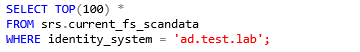
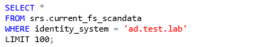
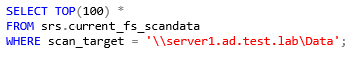
Example: Select file system data from a given identity system, limited to 100 entries.
SQL Server
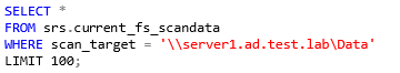
PostgreSQL
2.2.2 Scope by Server
Scoping by server is as simple as filtering by the server column in the srs.scan_targets table or in one of the supported srs.current_* views.
Also note that the server name may be case sensitive depending on the database collation.
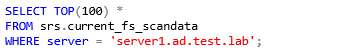
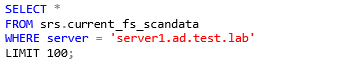
Example: Select all file system data from a specific server, limited to 100 entries.
SQL Server
PostgreSQL
2.2.3 Scope by Scan Target
Scoping by scan target is useful where a specific volume or share name is known.
Note that the scan target name may be case sensitive depending on the database collation.
Example: Select file system data from a particular scan target (share or volume) limited to 100 entries.
SQL Server
PostgreSQL
2.2.4 Scope by Directory
Scoping by a particular directory or folder requires the use of the hierarchical markers in the srs.scan_data table. These markers assist with determining parent and child folders as well as all subordinate file system entries for a given directory or set of directories.
|
Field |
Description |
Notes |
|---|---|---|
|
idx |
Entry index. |
Unique per scan. |
|
parent_idx |
Index of parent directory, share or DFS name space entry. |
For all sibling file system entries, they will have the same parent index. |
|
path_depth |
Current path depth relative to root path. |
The root path is always depth zero (0). Other paths such as shares may have the same depth as the root path, but can be distinguished by path_type.Entries occurring above the root path (such as DFS name spaces) will have a negative value. |
|
ns_left , ns_right |
Nested set indexes for current entry. |
Nested set markers provide a quick way to determine all subordinates for a given directory. See examples below for detail. |
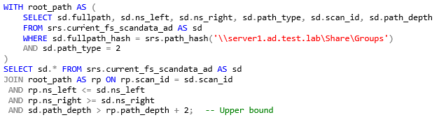
Example: Select all NTFS file system entries subordinate to, and including the specified target path.
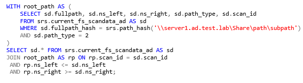
In this example, we are using two SELECT statements: one to get the information for the desired root path, and one to pull all subordinate entries along with the root path. Notice how the JOIN filter in the second SELECT statement uses not only the scan_id to limit the particular scan(s) of interest, but also uses the and fields to keep the data set limited to file entries in the folder hierarchy.
In the following diagram, an example of the nested set model calculations are shown with an example structure under \\Server\Share. In this example, exactly 1,000 file system entries exist, including files, folders, and the share itself.
Figure 2-1 Nested Set Calculations Example
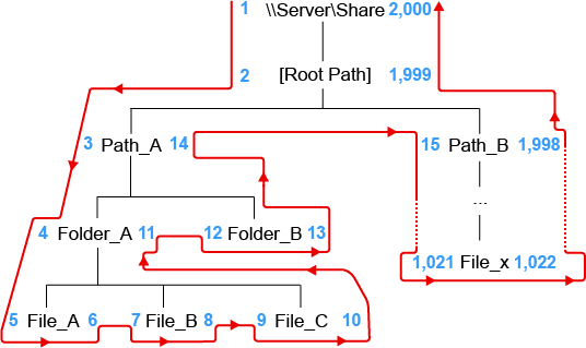
For each node in the scanned file structure, a left and right value are assigned. The values are assigned by traversing the imaginary path from the root down the left side of the structure, incrementing the values by one. Once a leaf node is encountered, the incrementing value continues, but is now assigned to
This process continues until the entire graph of the file structure has been traversed, and the root path is finally assigned the last number for its value.
The nested set model has the following characteristics, some of which are vital to hierarchical processing, such as determining subordinate objects:
-
The root path will always have a value of 1 and an value of 2n, where n = the total number of entries.
-
For any given container object (folder, share, etc.), all subordinate entries can be found by searching for all objects in the scan having an value greater than the container path’s value, and an value less than the container path’s value.
-
Nested set is generally the fastest method available in relational data models for retrieving all subordinate objects when representing hierarchical data.
For more information on the nested set model, see http://en.wikipedia.org/wiki/Nested_set_model.
2.2.5 Scope by Directory with Path Depth Limit
In addition to scoping by directory, it may be useful to start with a given path, but then only include subordinate paths within a given range below the selected path.
In this case, we make use of the same nested set model calculations seen in the previous section, but include the use of the parameter as well.
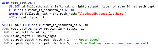
Example: Select all paths starting two levels below a given path.
This example is common when folder structures have managed content, such as collaborative or group folders, organized below division or department folders one or more layers deep. In order to pull all the content from just the group folders themselves, and not include the structural folders, we can make use of path depth, but assign the selected path to the root structural folder.
For a share organized as:
\\Server\Share\Groups\Departments\GroupA
The selected path could be \\Server\Share\Groups and the could be assigned to the root_path + 2 or greater, as in the SELECT statement above.
We could just as easily limit the depth of paths searched by adding another comparison of as a lower bounds:
2.2.6 Scope by Security Principal
Scoping by security principal is useful when querying for scan data specific to a given set of owners or trustees.
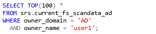
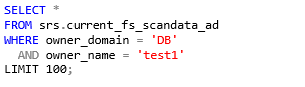
Example: Select all files for a given server owned by a specific AD user, limited to 100 entries.
SQL Server
PostgreSQL
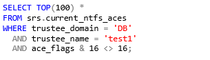
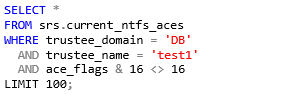
Example: Select all folders where a user is a direct trustee (not inherited) for NTFS, limited to 100 entries.
SQL Server
PostgreSQL
2.2.7 Basic Filtering
In addition to using filters to scope the range of scan data, basic filtering can also be used to limit the results to only records of interest.
The following is a list of basic filtering examples that may be used as starting templates for queries.
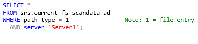
Filter by Path Type
In cases where aggregation or calculations against a discrete set of files is desired, it may be necessary to filter out any directories or shares first, since those entries contain size and name data that may skew the desired results.
Filter by File Extension
This example filters the set of file entries within a given directory structure to just those defined as media types.
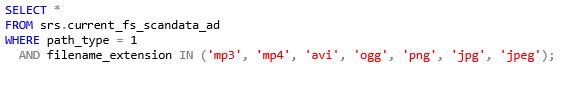
Note that for , all values should be lower case.
Filter by Date Range
This example selects all files on the specific server from November 1, 2013 midnight, through November 2, 2013 11:59 PM.
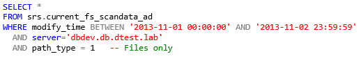
We can also use the familiar >= and <= comparison operators to accomplish the same:
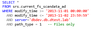
Note that the behavior of the BETWEEN operator is inclusive, not exclusive, to the parameters given.
Also it is important to note with date-time ranges, that a simple date such as ‘2013-11-02’ actually represents ‘2013-11-02 00:00:00’, so be careful to include 23:59:59 to the ending date as appropriate.
Finally, it is important to remember that all timestamps stored in the database are stored as UTC values, so consideration for time zone offsets may be needed.
Filter by File Name
This example shows how to filter by a given file name.
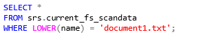
Note the use of the LOWER operator to force a case-insensitive search. Depending on the collation of the database instance and the database itself, this operator may be required.
For wildcard matches, the standard SQL flags _ and % can be used to represent a single or multiple characters.
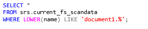
See the following links for database specific info regarding wildcards and other search patterns:
SQL Server: http://msdn.microsoft.com/en-us/library/ms190301
Postgres: http://www.postgresql.org/docs/9.3/static/functions-matching.html